
Dec 29, 2012 , by
Public Summary Month 11/2012
Contour following and profile estimation
Three different experiments have been performed to test the contour following algorithm.
The first one concerns the measurement of a linear profile with an artificial burr (Figs. 1-2).
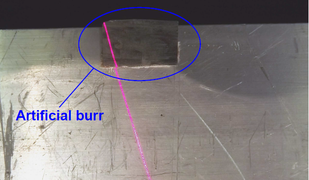
Fig. 1
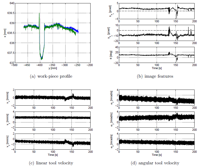
Fig. 2
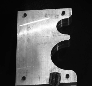
Fig. 3
The two other experiments show the performance of the contour following system in the case of a complex profile. In this case a work-piece with a profile characterised by a sequence of arcs of different radius has been selected (Fig. 3). The two experiments concern the contour following of the bigger and the smaller arc that characterise the work-piece. Though the geometry of the profile is more complex than in the first experiment, the control system exhibits almost the same performance (Fig. 4).
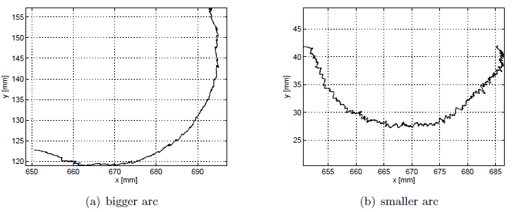
Fig. 4
The performance of the second part of the system, i.e. the triangulation algorithm, has been assessed in a realistic scenario, measuring the changes in the burr profile during a sequence of seven deburring trials. The experiment was organised as follows. First, different measurements of similar profiles have been taken and the nominal profile has been reconstructed. Then, the nominal profile has been used to drive the robot through seven different deburring trials, changing the depth of cut in the range from 0 to 1 mm (Figs. 5-6).
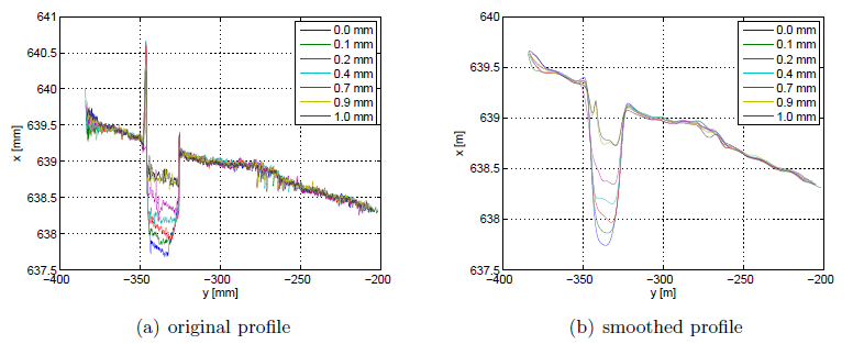
Fig. 5
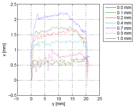
Fig. 6
Learning the tool path
Once a set of profiles of different work-pieces, characterised by the same nominal profile but affected by different burrs, has been acquired, the profiles are transformed into the distance space and a mean (or a median) profile is computed. The rationale behind this procedure is that if burrs are randomly distributed along the profiles of the different work-pieces, and if burr dimensions are negligible with respect to the work-piece dimensions, the mean profile approximates, with good accuracy, the nominal one.
An algorithm to generate a synthetic burr dataset has been developed. Interpolating the profiles reported in Figs. 6 and extracting the heigh of each point belonging to the actual profile with respect to the nominal one, seven models of burrs with the same length but different heights and a model of a segment of profile without burrs have been generated (Fig. 7).
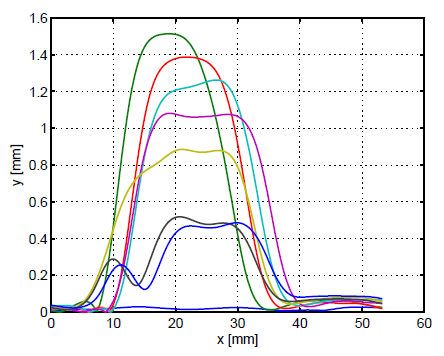
Fig. 7
Two different sets, each one composed of ten synthetic profiles, have been generated. The first one, reported in Fig. 8, is based on a linear nominal profile, the second one, shown in Fig. 9, on a circular nominal profile. The learning path procedure was applied to both sets, giving rise to the results reported in Figs. 10-11.
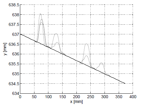
Fig. 8
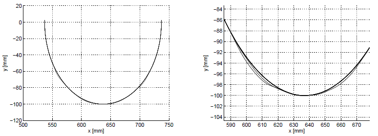
Fig. 9
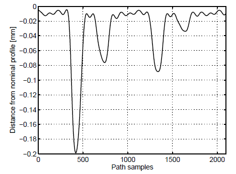
Fig. 10
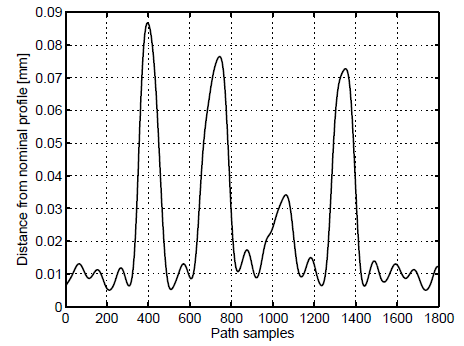
Fig. 11
Oct 19, 2012 , by
Public Summary Month 9/2012
System integration
Considering that the role of the vision system should be to determine the deburring profile and to measure the length and depth of burrs, as burrs in this kind of machining process are characterized by depth/length of 1-2 millimeters, the accuracy of the vision system should be in the order of tens of millimeters. If the profiles detected during subsequent experiments are compared on the basis of the image plane coordinates only the intrinsic camera parameters affect the precision; instead if the 3D coordinates of the profile are compared, the accuracy will be affected by the extrinsic camera parameters as well.
At this point, the accuracy of the self-calibration procedure used to determine the extrinsic camera parameters is not well enough to guarantee the required accuracy in the reconstruction of the 3D burr profile. A better self-calibration algorithm has thus been developed and is currently under validation.
Further, it must be considered that a reconstruction of the profile in the 3D space will be very useful, as it will give more information to the robot control system: the robot will be able to execute the path previously determined measuring the contact force (that gives an indirect measure of the burr length/depth) and thus deriving more information for the learning algorithm. On the other hand it will not be strictly necessary, as the profile reconstructed in the image plane should be sufficient to measure the burr characteristics during subsequent deburring experiments (and this represents the minimal amount of information required by the learning system).
Here can be found two video of a scan from the image processing side and from the robot side.
Learning the deburring path
A paper concerning the study developed to learn a deburring path has been submitted to ICRA 2013.
Aug 13, 2012 , by
Public Summary Month 7/2012
Visual servoing control for contour following
To support the scanning procedure a visual servoing control able to move the robot along the deburring path, keeping the camera (and the laser) at a fixed distance from the wheel and centered on the edge, is required (Fig. 1).
|
|
| Figure 1 - Architecture of the visual servoing controller |

At each camera frame, ten points are measured on the deburring edge by way of a set of edge detectors, and the least square fitting line is computed. To ensure robustness the 3-parameters line equation and a method to automatically discard outliers are used.
The orientation of this line and the distance from the camera optical center are fed into a visual servoing loop that controls the motion of the robot. In particular, this control acts on the absolute velocity of the camera frame vcx, vcy, vcz and ωcz to keep the optical axis on the edge and one of the axis of the image frame parallel to the contour. Further, the velocity along the optical axis is used to keep the desired distance between the image plane and the wheel surface. To accomplish such a decomposition of the robot motion in the xy-plane and along the optical axis, the partitioned visual servoing control methodology has been selected.
Preliminary analysis of the deburring profile have been performed, exploiting the control system just described to drive the robot along the path (Fig. 2).
 |
 |
 |
 |
 |
 |
| Figure 2 - Six frames extracted from an edge analysis | ||
The results of one of these experiments are reported in Figs. 3-5. In particular, Figs. 3 show the x, y-errors on the image plane (the components of the vector e) and the orientation error. Note that these errors are very small (apart from the initial transient that represents the approach to the contour).
On the other hand, Figs. 4 show the control variables.
Finally, Fig. 5 shows the reconstructed deburring profile.
 |
 |
 |
|
| Figure 3 - The visual servoing errors in the image plane | |
 |
 |
 |
|
| Figure 4 - The control actions generated by the visual servoing laws | |
 |
| Figure 5 - The deburring proflle |
Walk-through programming in contact
An hybrid admittance-force control scheme, that allows the walk-through programming in free motion and in contact with and hard surface, has been realised and tested in simulation.
The behavior of the control system is as follows: during the walk-through programming in free motion the robot in controlled by way of the admittance filters, when a contact is detected the surface normal is immediately estimated and the control along the normal direction is switched to force control (in order to ensure the contact at a desired force value).
Jul 8, 2012 , by
Public Summary Month 5/2012
Walk-through programming
The problem of walk-through programming in contact with an hard surface is still under studying.
The main concerns are related to the implementation of a robust algorithm to detect the contact and estimate the normal to the surface.
Wheel localisation and burr analysis
To localise the wheel a camera mounted on top of the working area is usually adopted. Further, in industrial applications the valve hole is the feature usually adopted to localise the wheel. Nevertheless, we decided to mount the camera on the robot shoulder considering the following advantages:
- it is a simpler and more compact solution, that does not require any additional frame to support the camera (that could represent a dangerous obstacle in the robot workspace);
- it allows for a bigger and less occluded field of view (we do not need to ensure that the arm does not occlude the wheel or the valve hole);
- the shoulder camera can be used as an additional sensor during the deburring operation or as a recording device.
The shoulder mountig, however, entails disadvantages as well: the majority of the time the valve hole is occluded or difficult to detect due to shadows or poor illumination. The pictures taken by the camera from different robot positions suggest that the bolt holes (and their positions with respect to the wheel) represent a set of robust features to localise the wheel.
Concerning burr analysis, it must be noticed that the burr profile is estimated directly on the image plane (no extrinsic camera parameters need to be calibrated). Nonetheless, a calibration of the laser with respect to the camera and a validation of the system precision are of upmost importance.
The following tables show the results of this validation.
Each table compares the results obtained with two algorithms, A e B, and the one computed as the mean of the previous ones. In algorithm A the position of each point of the laser line is determined looking for the point, along a perpendicular to the laser, that maximises the brightness. On the other hand, algorithm B determines the position of the points on the line as the mean value between an upper and a lower threshold on the derivative of the brightness.
The first table concerns measurements of the distance along the z (focal) axis of the camera frame, between the center of the camera frame and the surface of a calibration object, a stair of 9 steps, each with an height of 1 cm.
Mean and standard deviation were computed processing 100 pictures, taken with slightly different light conditions.
The table shows a very low variance in the measurements. It must be noticed, however, that there are small errors in the distances (the nominal distance between two consecutive steps is 1 cm) due to the fact that the distance between the camera and the laser was not corrected with an accurate calibration.
|
Algorithm A |
Algorithm B |
Mean |
|||
|
Mean |
Standard deviation |
Mean |
Standard deviation |
Mean |
Standard deviation |
|
0.4851 |
0.000000 |
0.4851 |
0.000125 |
0.4851 |
0.000062 |
|
0.4746 |
0.000000 |
0.4747 |
0.000046 |
0.4746 |
0.000023 |
|
0.4642 |
0.000000 |
0.4642 |
0.000049 |
0.4642 |
0.000024 |
|
0.4537 |
0.000081 |
0.4537 |
0.000235 |
0.4537 |
0.000134 |
|
0.4432 |
0.000000 |
0.4433 |
0.000159 |
0.4433 |
0.000080 |
|
0.4331 |
0.000038 |
0.4329 |
0.000021 |
0.4330 |
0.000024 |
|
0.4229 |
0.000000 |
0.4227 |
0.000099 |
0.4228 |
0.000049 |
|
0.4123 |
0.000021 |
0.4124 |
0.000233 |
0.4123 |
0.000116 |
|
0.4022 |
0.000000 |
0.4023 |
0.000150 |
0.4022 |
0.000056 |
The last table shows the z distances measured on a part of the wheel. In this case there is no ground truth, but the small standard deviations demonstrate that accurate measures can be obtained even on a rough metal surface.
|
Algorithm A |
Algorithm B |
Mean |
|||||
|
Mean |
Standard deviation |
Mean |
Standard deviation |
Mean |
Standard deviation |
||
|
0.4338 |
0.000000 |
0.4335 |
0.000024 |
0.4337 |
0.000012 |
||
|
0.4340 |
0.000082 |
0.4335 |
0.000024 |
0.4337 |
0.000044 |
||
|
0.4375 |
0.000025 |
0.4375 |
0.000026 |
0.4375 |
0.000025 |
||
|
0.4435 |
0.000027 |
0.4435 |
0.000027 |
0.4435 |
0.000027 |
||
|
0.4452 |
0.000027 |
0.4453 |
0.000027 |
0.4453 |
0.000027 |
||
|
0.4436 |
0.000027 |
0.4436 |
0.000027 |
0.4436 |
0.000027 |
||
|
0.4381 |
0.000026 |
0.4381 |
0.000030 |
0.4381 |
0.000027 |
||
|
0.4334 |
0.000028 |
0.4330 |
0.000028 |
0.4332 |
0.000028 |
||
|
0.4331 |
0.000028 |
0.4324 |
0.000092 |
0.4328 |
0.000055 |
||
Apr 15, 2012 , by
Public Summary Month 3/2012
Walk-through programming
The programming mode has been realised through a set of admittance controllers.

It must be noticed that the tests reaveal that the classical implementation of the walk-through programming mode does not allow for motion in contact with a surface. It turns out that realising the walk-through programming in contact with a hard surface (with a single force/torque sensor) is a quite challenging operation, but it is also uf upmost importance not only for this project but, for example, in many surgical robotics applications. We are still studying this problem.

Wheel localisation and burr analysis
A set of specifications for the two camera systems (one for wheel localisation, the other one for burr analysis) has been identified. Within the end of the month two cameras and a laser stripe will be available for thesting the image processing algorithms.
Some mechanical devices that can artificially mimic a contour with a burr have been also sketched and will be soon realised (see the picture below).